SciPy - Normal Distribution

Normal (Gaussian) Distribution is a probability function that describes how the values of a variable are distributed. It is a symmetric distribution about its mean where most of the observations cluster around the mean and the probabilities for values further away from the mean taper off equally in both directions. It is the most important probability distribution function used in statistics because of its advantages in real case scenarios. For example, the height of the population, measurement errors etc.

The probability density function (pdf) of normal distribution is defined as:

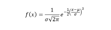
Where, μ is the mean or expectation of the distribution and σ is the standard deviation of the distribution.

An normal distribution has mean μ and variance σ². A normal distribution with μ=0 and σ=1 is called standard normal distribution.

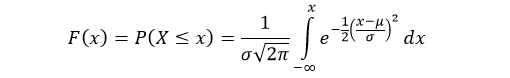
The cumulative distribution function (cdf) evaluated at x, is the probability that the random variable (X) will take a value less than or equal to x. The cdf of normal distribution is defined as:

The scipy.stats.norm contains all the methods required to generate and work with a normal distribution. The most frequently methods are mentioned below:

Syntax

scipy.stats.norm.pdf(x, loc=0, scale=1)
scipy.stats.norm.cdf(x, loc=0, scale=1)
scipy.stats.norm.ppf(q, loc=0, scale=1)
scipy.stats.norm.rvs(loc=0, scale=1, size=1)

Parameters

norm.pdf()

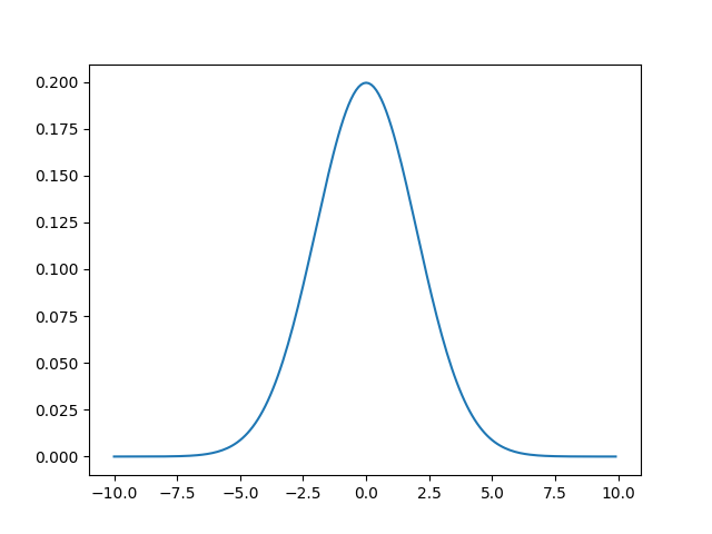
The norm.pdf() function measures probability density function (pdf) of the distribution.

from scipy.stats import norm
import matplotlib.pyplot as plt
import numpy as np

#creating an array of values between
#-10 to 10 with a difference of 0.1
x = np.arange(-10, 10, 0.1)
   
y = norm.pdf(x, 0, 2)
   
plt.plot(x, y) 
plt.show()

The output of the above code will be:

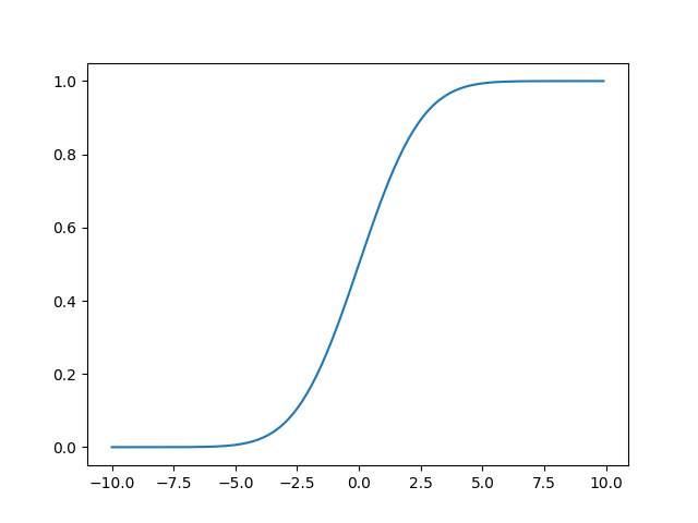
norm.cdf()

The norm.cdf() function returns cumulative distribution function (cdf) of the distribution.

from scipy.stats import norm
import matplotlib.pyplot as plt
import numpy as np

#creating an array of values between
#-10 to 10 with a difference of 0.1
x = np.arange(-10, 10, 0.1)
   
y = norm.cdf(x, 0, 2)
   
plt.plot(x, y) 
plt.show()

The output of the above code will be:

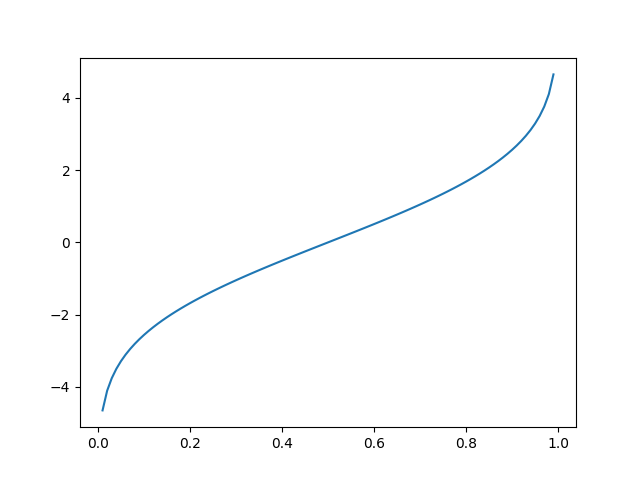
norm.ppf()

The norm.ppf() function takes the probability value and returns cumulative value corresponding to probability value of the distribution.

from scipy.stats import norm
import matplotlib.pyplot as plt
import numpy as np

#creating an array of probability from
#0 to 1 with a difference of 0.01
x = np.arange(0, 1, 0.01)
   
y = norm.ppf(x, 0, 2)
   
plt.plot(x, y) 
plt.show()

The output of the above code will be:

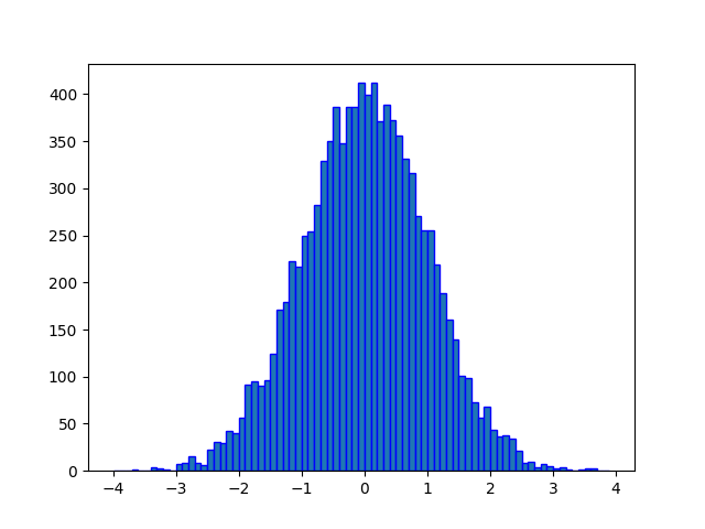
norm.rvs()

The norm.ppf() function generates an array containing specified number of random numbers of the given normal distribution. In the example below, a histogram is plotted to visualize the result.

from scipy.stats import norm
import matplotlib.pyplot as plt
import numpy as np

#fixing the seed for reproducibility
#of the result
np.random.seed(10)

#creating a vector containing 10000
#normally distributed random numbers
y = norm.rvs(0, 1, 10000)

#creating bin
bin = np.arange(-4,4,0.1)  

plt.hist(y, bins=bin, edgecolor='blue') 
plt.show()

The output of the above code will be: